Kelly Criterion: Optimal Position Sizing for Systematic Traders
The Kelly Criterion tells you exactly how much capital to risk per trade to maximize the long-run growth rate of your portfolio — not just make it bigger faster, but avoid the ruin that comes from betting too large. It is the mathematical bridge between having an edge and actually compounding that edge over time.
Try it live: AlgoDrill's Kelly Criterion + Expectancy calculator runs in your browser — enter your win rate and average win/loss to get the Kelly fraction instantly.
The Formula
The Kelly formula for a binary win/loss bet (the version most useful for discrete trading strategies) is:
Equivalently, with win probability p, average win W, and average loss L:
- f* = (p × W − (1−p) × L) / W — or more intuitively:
- f* = Expectancy / Average Win — the edge per dollar you can win, divided by what you'd win per dollar bet.
A positive Kelly fraction means you have a positive-expectancy edge. A zero or negative result means stop trading the setup — no amount of position sizing fixes a losing strategy.
Derivation: Why Geometric Growth?
Kelly's insight (from his 1956 Bell System paper) was to maximize geometric growth rate, not expected value. Expected value maximization leads to ruin: bet everything on 51% odds, and one streak wipes you out even though the expected value is positive.
The growth rate of a portfolio over N bets is:
Differentiating G with respect to f and setting to zero yields the Kelly fraction. The curve is concave — there is a unique maximum, and betting more than Kelly reduces long-run growth. Betting 2× Kelly achieves the same expected growth as betting 0 (staying in cash). This asymmetry is called the Kelly asymmetry: overbetting is catastrophic; underbetting is merely suboptimal.
Python Implementation
def kelly_fraction(win_rate: float, avg_win: float, avg_loss: float) -> dict:
    """
    Compute Kelly fraction and derived metrics.

    Args:
        win_rate: fraction of trades that are winners (e.g., 0.55 for 55%)
        avg_win:  average profit on winning trades (positive, e.g., 150.0)
        avg_loss: average loss on losing trades (positive magnitude, e.g., 100.0)

    Returns dict with kelly_f, expectancy, payoff_ratio.
    """
    if avg_win <= 0 or avg_loss <= 0:
        raise ValueError("avg_win and avg_loss must be positive")
    if not (0 < win_rate < 1):
        raise ValueError("win_rate must be between 0 and 1")

    loss_rate = 1.0 - win_rate
    payoff_ratio = avg_win / avg_loss                   # W/L
    expectancy = win_rate * avg_win - loss_rate * avg_loss  # E[trade]
    kelly_f = expectancy / avg_win                      # f* = E/W

    return {
        "kelly_f":      round(kelly_f, 4),
        "half_kelly_f": round(kelly_f / 2, 4),
        "expectancy":   round(expectancy, 4),
        "payoff_ratio": round(payoff_ratio, 4),
    }

# Example: 55% win rate, avg win $150, avg loss $100
result = kelly_fraction(0.55, 150, 100)
# kelly_f=0.25  →  risk 25% of capital per trade
# half_kelly_f=0.125  →  practitioners use this
# expectancy=$37.50 per trade
print(result)
The example above — 55% win rate, $150 average win, $100 average loss — yields a full Kelly of 25%. Most practitioners immediately halve this to 12.5% (half-Kelly) to reduce volatility without sacrificing much growth.
Fractional Kelly in Practice
The full Kelly fraction is the theoretical maximum, but real trading deviates from the model assumptions in three ways that make full Kelly dangerous:
- Estimation error: Your historical win rate and average win/loss are noisy estimates. If true win rate is 52% but you estimated 55%, full Kelly is 1.5× the true optimal — in the dangerous overbetting zone.
- Non-stationarity: Win rates and payoffs change with market regime. A strategy that was 55% win rate in 2022 may be 48% in 2024. Kelly computed on stale data will oversize.
- Path risk: Even with accurate estimates, full Kelly produces maximum-growth drawdowns that are psychologically unsustainable (often 30–50%). You will deviate from the strategy under drawdown before the edge compounds.
The practical answer is fractional Kelly:
| Fraction | Growth rate | Max expected drawdown | Typical use case |
|---|---|---|---|
| Full Kelly (1.0×) | Maximum | High (often 30–50%) | Theoretical benchmark only |
| Half-Kelly (0.5×) | ~75% of max | Moderate (often 15–25%) | Most quant practitioners |
| Quarter-Kelly (0.25×) | ~44% of max | Low (often 8–12%) | High estimation uncertainty |
| Fixed fractional (e.g. 1–2%) | Suboptimal but stable | Capped by rule | Retail, early-stage strategies |
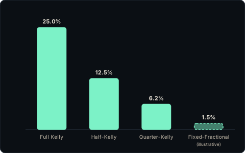
code-examples.ts. Fixed-Fractional: the "typical practice" range from the table above (1-2%), illustrative, not from that run.Half-Kelly captures roughly 75% of Kelly growth rate while cutting drawdowns roughly in half. It is the most common practitioner choice because the growth sacrifice is modest but the path-risk reduction is substantial.
Kelly and Sharpe: The Connection
For a continuous strategy (many small bets), the Kelly-optimal exposure is approximately the mean return divided by the return variance — equivalently, the Sharpe Ratio divided by the volatility (both measured over the same period). Specifically, for normally distributed daily returns:
Note that this typically implies leverage, not a small capital fraction. A strategy with annualized Sharpe 1.0 has a daily Sharpe of 1/√252 ≈ 0.063; at 1% daily volatility that is μ ≈ 0.063% per day, so f* = μ/σ² ≈ 0.00063 / 0.0001 ≈ 6.3 — a 6.3× levered position. Full continuous Kelly exceeding 1× capital even for a genuinely good strategy is one more reason practitioners run fractional Kelly: estimation error and fat tails make full-Kelly leverage unsurvivable in practice.
Failure Modes and When Kelly Breaks Down
Kelly is a growth-rate maximizer, not a risk manager. Several situations cause it to give dangerously wrong answers:
- Fat tails / extreme losses: Kelly assumes bounded losses. If a single trade can lose more than your average loss (gap risk, unlimited short, leverage blow-up), full Kelly can produce ruin-level sizing. Always cap your maximum loss exposure independently of Kelly.
- Non-independent trades: Kelly assumes each trade is statistically independent. Correlated positions (multiple long equities in a crash) compound losses faster than the model predicts. Compute Kelly on the portfolio return stream, not individual positions.
- Small sample estimates: With fewer than ~30 trades in your history, win rate and average payoff estimates have wide confidence intervals. Use half- or quarter-Kelly aggressively until you have 100+ trades of data.
- Regime change: A mean-reversion edge discovered in 2020 may disappear in a trending regime. Kelly sizing computed on the discovery period will oversize in the out-of-sample regime.
The Kelly number is an upper bound, not a target. It answers "what is the maximum fraction that avoids long-run ruin?" Not "what fraction should I use?" In practice: start at quarter-Kelly or fixed 1–2%, compute Kelly as a sanity check, and only approach half-Kelly once you have 100+ out-of-sample trades confirming the edge estimate.
Worked Example: Evaluating a Strategy
import numpy as np

# 200-trade history from a mean-reversion strategy on ES futures
trade_pnl = np.array([...])  # your actual P&L array

wins = trade_pnl[trade_pnl > 0]
losses = trade_pnl[trade_pnl < 0]

win_rate   = len(wins) / len(trade_pnl)     # 0.58
avg_win    = wins.mean()                    # $210
avg_loss   = abs(losses.mean())             # $145

result = kelly_fraction(win_rate, avg_win, avg_loss)
# kelly_f=0.29   →  29% full Kelly
# half_kelly_f=0.145  →  14.5% half-Kelly
# expectancy=$60.90 per trade

# With $50,000 account, half-Kelly = risk $7,250 per trade
# At 10-point stop (ES = $50/point), position size = 14.5 contracts
# In practice, round down to 14 and add a hard $7,000 daily loss limit
account_size = 50_000
max_risk_per_trade = account_size * result["half_kelly_f"]
print(f"Risk per trade: ${max_risk_per_trade:,.0f}")
Frequently Asked Questions
- What does a negative Kelly fraction mean?
- A negative Kelly result means your strategy has negative expectancy — the edge is working against you, not for you. No position sizing fixes a losing edge. If your Kelly is negative, stop trading the setup and investigate why: look for data errors, look-ahead bias, or a regime change that invalidated the backtest.
- Why do most quant traders use half-Kelly instead of full Kelly?
- Full Kelly maximizes long-run geometric growth but produces extreme drawdowns (often 30–50%) along the way. Most traders cannot sustain those drawdowns emotionally or operationally — they deviate from the strategy before the edge compounds. Half-Kelly captures roughly 75% of Kelly growth while cutting drawdowns roughly in half. The math says full Kelly is optimal; the psychology and estimation-error risk say half-Kelly is more robust in practice.
- Can I use Kelly Criterion for multiple simultaneous positions?
- Yes, but you need to compute Kelly on the portfolio's aggregate return stream, not on each position individually. Summing individual Kelly fractions ignores correlation — two correlated long positions in a crash behave like one large position, not two independent ones. The multi-asset Kelly formula accounts for the covariance matrix of returns. Alternatively, apply a conservative flat multiplier (0.5× or 0.25×) to all individual Kelly fractions to proxy for correlation.
- How many trades do I need before Kelly estimates are reliable?
- At 30 trades, the 95% confidence interval on your win rate is roughly ±18 percentage points (binomial). At 100 trades, it is still roughly ±10 points. For Kelly to be meaningful, most practitioners want at least 50–100 trades of out-of-sample history. With fewer trades, use fixed fractional sizing (1–2% per trade) and treat Kelly as a long-term monitoring metric rather than a real-time sizing input.
- Does Kelly work for options or leveraged instruments?
- The standard binary Kelly formula assumes bounded payoffs (you win W or lose L). Options have asymmetric payoffs (a long option can return many multiples of risk; a short option has theoretically unlimited loss). For options, you need the generalized Kelly formula that integrates over the full payoff distribution. For practical purposes: for defined-risk spreads, plug in max profit and max loss; for undefined-risk positions, Kelly is dangerous — hard caps on notional exposure matter more than Kelly optimization.
- Is Kelly Criterion related to the Sharpe Ratio?
- Yes, they are connected through portfolio theory. For a strategy with normally distributed returns, the Kelly fraction (as a fraction of capital per unit time) approximates mean return / return variance, which is also the Sharpe Ratio divided by volatility. A higher Sharpe strategy has a higher Kelly fraction — both metrics reward edge per unit of risk. The Sharpe Ratio measures risk-adjusted return; Kelly measures how to size to exploit that return most efficiently.
Run the Kelly Criterion calculator on your own trade history — no sign-up, no data leaves your browser.
Open Kelly Calculator → Drill Risk & Sizing Flashcards →