Time Series Momentum, Replicated

Moskowitz, T. J., Ooi, Y. H., & Pedersen, L. H. (2012). Time Series Momentum. Journal of Financial Economics, 104(2), 228–250.

Paper (PDF) · SSRN · Runnable backtest pattern

The claimed edge

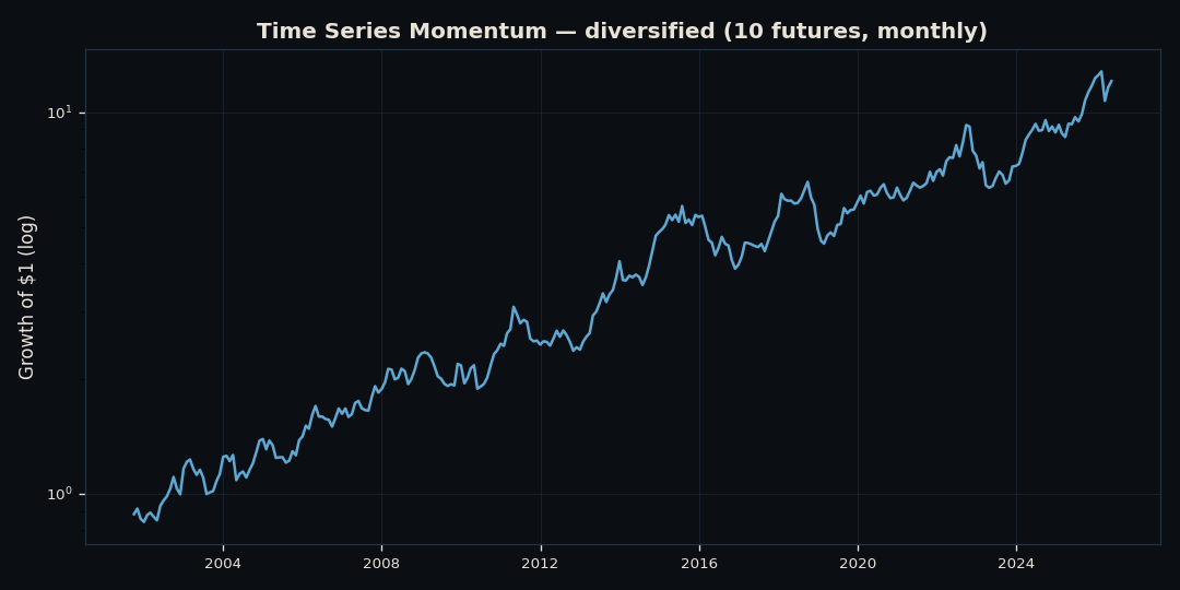
An instrument's own past 12-month return predicts its next-month return. Go long if the trailing year was positive, short if negative, size each position inversely to its volatility, hold a month, rebalance. Averaged across 58 futures spanning equities, bonds, commodities, and currencies, the paper reports a diversified gross Sharpe of roughly 1.2 (1985–2009), strongest in extreme markets. This is the academic foundation under the trend-following archetype the deck drills.

What we tested

Universe: 10 liquid futures across 4 asset classes (ES, NQ, YM, CL, GC, SI, ZN, ZB, 6E, 6J) — a free-data subset of the paper's 58.
Rules: sign(trailing 12-month return) → long/short, position scaled to a 40% ex-ante vol target, 1-month hold, monthly rebalance. Diversified factor = equal-weight average across instruments. No look-ahead.
Engine: the diversified factor is a vectorized pandas calc; a single-instrument long/short illustration (ES) runs through backtesting.py so the rule is readable on one contract.

Result (2000–2026)

Metric	Diversified TSM (10 futures)
Annualized return	10.6%
Annualized volatility	18.7%
Sharpe	0.63
Sortino	0.64
Max drawdown	−31.5%
Calmar	0.34

Growth-of-$1 equity curve of the diversified Time Series Momentum portfolio, 2000 to 2026, log scale. — Diversified TSM portfolio (10 futures), monthly rebalanced, log scale.

Did it hold up? Validation against AQR

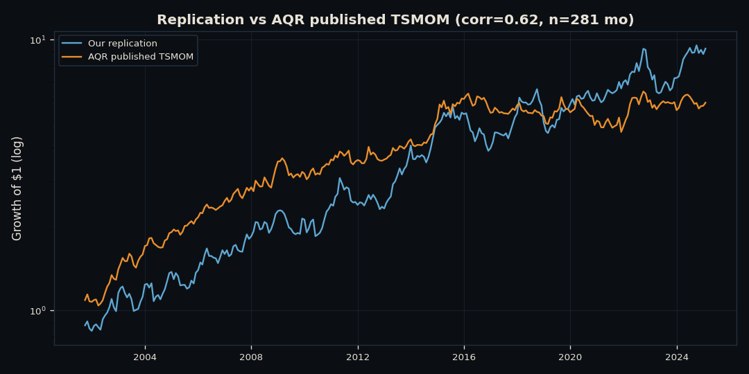
AQR publishes the original paper's TSMOM factor returns. Our 10-instrument replication's monthly returns correlate 0.62 with AQR's published 58-instrument factor across 281 overlapping months. That's the key result: the signal replicates — we're capturing the same effect — even with a smaller universe and rougher data.

Overlay of our replication's cumulative return versus AQR's published TSMOM factor, showing they track each other. — Our replication vs. AQR's published TSMOM factor (monthly-return correlation 0.62).

Where it fell short — honestly

Our 0.63 Sharpe is well below the paper's ~1.2. The gap is real and explainable, not a bug:

Post-publication decay. Trend-following / TSM weakened markedly after ~2009 (the CTA "lost decade," roughly 2011–2019). The paper's sample ended in 2009; ours includes the drawdown. The 0.62 correlation says the signal still works; the payoff shrank.
Continuous front-month futures, no roll adjustment. Free data (yfinance) serves unadjusted continuous contracts. Momentum P&L is sensitive to roll yield, so unadjusted series understate trend returns.
10 instruments vs 58. Less diversification → lower risk-adjusted return.
Gross factor. The diversified factor excludes transaction costs (the single-instrument illustration includes a 2bp commission).

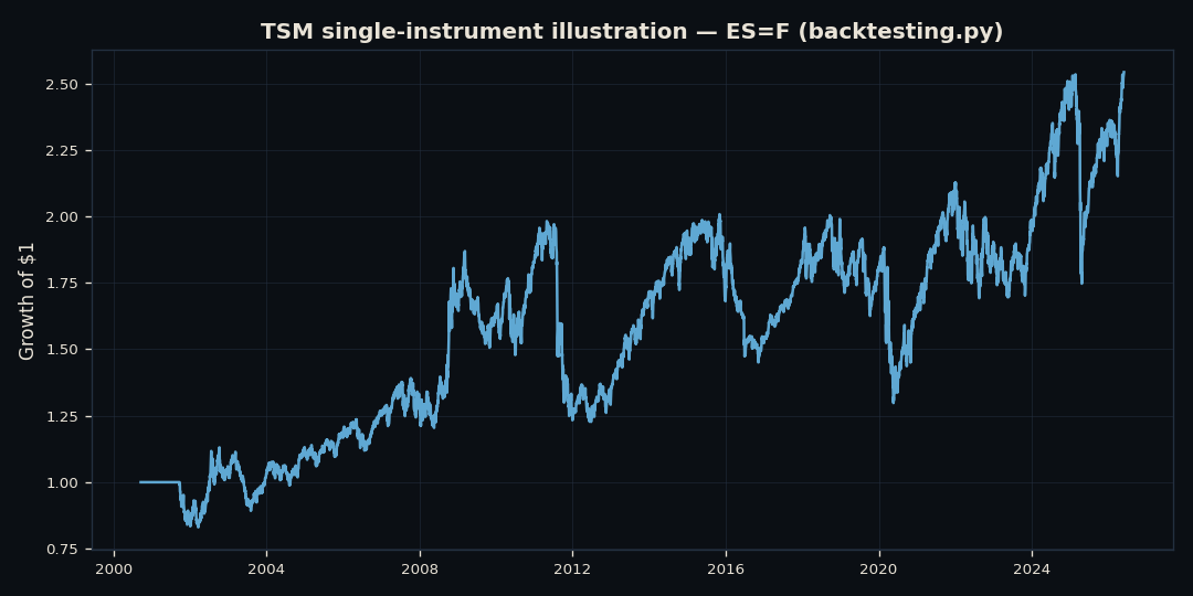
The honest takeaway: the effect is real and replicates out-of-sample, but its magnitude has decayed and free data understates it. That's a more useful result than a cherry-picked Sharpe — and exactly why we publish the code.

Equity curve of the single-instrument backtesting.py illustration on the E-mini S&P 500. — Single-instrument illustration (ES, `backtesting.py`): the same long/short rule on one contract.

Rebuild it and verify

Don't take our word for any of this — every rule is stated above: universe, signal, sizing, rebalance, and costs. The same pattern — fetching data, computing a trend signal, running the loop, reading the stats — is walked through line by line in our code pages.

SMA-crossover backtest walkthrough · Reading backtest stats · Drill the trend-following archetype: algodrill.app/study

This is a historical backtest; past results, especially decayed ones, do not predict future returns.