Sharpe Ratio: Formula, Benchmarks, and Python Implementation
The Sharpe Ratio is the single most widely reported risk-adjusted return metric in systematic trading. It answers one question: how much excess return does this strategy earn per unit of risk? A strategy returning 30% annually sounds impressive — until you learn it does so with 40% annual volatility. A strategy returning 10% with 5% volatility is far more efficient. The Sharpe Ratio quantifies that difference.
The Formula
For a return series R over a given period, with risk-free rate Rf:
The formula is deceptively simple. Three implementation choices determine whether your computed Sharpe matches published figures:
- Risk-free rate: Use the period-equivalent rate, not the annualized rate. If your returns are daily, divide the annual risk-free rate by 252 (or use 0 for simplicity — most practitioners omit Rf for short-term comparisons).
- Sample vs. population std dev: Use sample standard deviation (denominator N−1) for realistic estimates. Using population std dev (N) understates volatility, inflating the ratio.
- Annualization: Multiply the period Sharpe by the appropriate annualization factor (see table below) so ratios across different periodicities are comparable.
Annualization
Raw Sharpe ratios computed on daily data are far smaller than those on monthly data because daily returns are more volatile relative to the mean. To make ratios comparable, multiply by the square root of the number of periods per year:
The square-root rule follows from the assumption that returns are i.i.d. (independently and identically distributed) — mean scales linearly with time, variance scales linearly, and standard deviation scales with the square root. When returns exhibit autocorrelation (each return is correlated with the previous one), this assumption breaks down and the annualized Sharpe is overstated; see the failure modes section below.
Interpretation Benchmarks
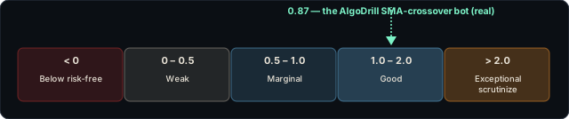
| Annualized Sharpe | Verdict | Notes |
|---|---|---|
| < 0 | Below risk-free | Strategy underperforms cash on a risk-adjusted basis. Stop. |
| 0 – 0.5 | Weak | S&P 500 long-run Sharpe ≈ 0.4–0.5. No advantage over passive investing. |
| 0.5 – 1.0 | Marginal | Covers execution costs but leaves little margin. Commissions can flip it negative. |
| 1.0 – 2.0 | Good | Target range for retail systematic strategies. Worth the complexity. |
| > 2.0 | Exceptional — scrutinize | Often indicates look-ahead bias or overfitting in backtests. Rare in live trading. |
code-examples.ts.Python Implementation
import math

def sharpe_ratio(returns: list[float], risk_free_rate: float = 0.0) -> float:
    """
    Compute the period Sharpe Ratio (not annualized).

    Args:
        returns:        list of period returns as decimals (e.g., 0.01 for 1%)
        risk_free_rate: period risk-free rate (use 0 to omit)

    Returns the Sharpe Ratio for the period. Multiply by an annualization
    factor to get the annualized Sharpe.
    """
    n = len(returns)
    if n < 2:
        raise ValueError("Need at least 2 data points")

    mean_r = sum(returns) / n
    excess  = mean_r - risk_free_rate
    variance = sum((r - mean_r) ** 2 for r in returns) / (n - 1)  # sample std dev
    std = math.sqrt(variance)

    return 0.0 if std == 0 else excess / std


ANNUALIZATION = {
    "daily":   math.sqrt(252),
    "weekly":  math.sqrt(52),
    "monthly": math.sqrt(12),
    "annual":  1.0,
}

def annualized_sharpe(returns: list[float], periodicity: str = "daily",
                       risk_free_rate: float = 0.0) -> float:
    factor = ANNUALIZATION.get(periodicity, ANNUALIZATION["daily"])
    return sharpe_ratio(returns, risk_free_rate) * factor
Example: Evaluating a Strategy on a Return Series
import numpy as np

# 252 daily returns (one year) from a mean-reversion strategy
daily_returns = np.array([...])  # your actual return array

s = annualized_sharpe(daily_returns.tolist(), periodicity="daily")
print(f"Annualized Sharpe: {s:.3f}")
# e.g., 1.42 → strong; 0.38 → weak

# Risk-free adjustment (e.g., 5% annualized T-bill rate):
daily_rfr = 0.05 / 252
s_adjusted = annualized_sharpe(daily_returns.tolist(), periodicity="daily",
                                risk_free_rate=daily_rfr)
print(f"Risk-free-adjusted Sharpe: {s_adjusted:.3f}")
NumPy shortcut: np.mean(r) / np.std(r, ddof=1) * np.sqrt(252) gives the annualized Sharpe for daily returns without a risk-free rate. This is the form most quant libraries use internally.
Sharpe vs. Other Risk Metrics
| Metric | What it penalizes | When to prefer it |
|---|---|---|
| Sharpe Ratio | Total volatility (up and down) | Default choice; symmetrical payoff strategies |
| Sortino Ratio | Downside volatility only | Positively-skewed strategies; trend-following where upside runs are desirable |
| Calmar Ratio | Max drawdown (not volatility) | CTA-style funds; strategies where drawdown depth matters more than daily vol |
| Information Ratio | Tracking error vs. benchmark | Long-only equity strategies benchmarked against an index |
Sharpe and Sortino diverge most on options strategies and trend-following. A covered-call strategy harvests premium steadily but blows up in crashes — high Sharpe, low Sortino. Trend-following has frequent small losses but large wins — lower Sharpe, higher Sortino relative to Sharpe. Computing both captures these asymmetries. AlgoDrill's calculators compute both simultaneously.
Failure Modes: When Sharpe Misleads
- Non-normality (fat tails): The Sharpe formula is derived under the assumption of normally distributed returns. Strategies with heavy-tailed or negatively-skewed return distributions (selling options, binary bets) can show high Sharpe while carrying hidden ruin risk. A strategy with Sharpe 2.0 that blows up once every five years has an expected long-run Sharpe far below 2.0. Always compute kurtosis and skew alongside Sharpe.
- Autocorrelation inflation: If returns are positively autocorrelated (today's return predicts tomorrow's), the i.i.d. assumption underlying the √T annualization breaks down. The computed standard deviation understates true risk, inflating Sharpe. Monthly-rebalanced portfolios often exhibit this. The Ljung-Box test detects autocorrelation; Lo (2002) provides an autocorrelation-corrected Sharpe estimator.
- Look-ahead bias: Using future data in the signal calculation (even accidentally — e.g., using the close price of the bar on which the signal fires) inflates Sharpe dramatically. One tick of look-ahead on a high-frequency strategy can produce a Sharpe of 10+ from pure noise. Walk-forward validation is the only reliable diagnostic.
- Short sample bias: Sharpe estimated on fewer than 60 daily observations has a standard error wide enough to contain zero for most reasonable strategies. Bailey and López de Prado's Probabilistic Sharpe Ratio adjusts for this — it asks "what is the probability that the true Sharpe exceeds a benchmark?" given the sample size and skew.
- Survivorship bias: Backtests on a stock universe that excludes delisted companies overstate Sharpe because the worst-performing assets are missing. Use point-in-time constituent data or a survivorship-bias-free data source.
Rule of thumb: if a strategy's backtested Sharpe exceeds 3.0 — especially with a short sample, many parameters, or no out-of-sample holdout — assume the number is wrong until proven otherwise. Exceptional Sharpe is far more likely to be an artifact of methodology than genuine alpha.
Sharpe and Position Sizing
The Sharpe Ratio does not directly tell you how to size positions — that is the Kelly Criterion's domain. But the two metrics are connected: for a strategy with normally distributed returns, the Kelly fraction is approximately proportional to the Sharpe Ratio divided by volatility. A higher Sharpe strategy supports larger Kelly sizing for the same volatility level. A low-Sharpe, high-volatility strategy has a small Kelly fraction — the market is offering little edge per unit of risk, so you should bet little.
The practical relationship: compute Sharpe first to evaluate whether the strategy has any edge worth sizing. Then use Kelly to determine how much to size it. A strategy with Sharpe below 0.5 is unlikely to survive real-world execution costs even at optimal Kelly sizing.
Frequently Asked Questions
- What is a good Sharpe Ratio for algorithmic trading?
- Above 1.0 is generally considered good for a live trading strategy; above 2.0 is exceptional and warrants scrutiny for look-ahead bias or overfitting. Below 0.5 means the strategy barely compensates for its volatility — commissions and slippage will likely push it negative live. The S&P 500 long-run Sharpe is roughly 0.4–0.5, so any systematic strategy should comfortably beat that to justify the execution complexity.
- How do I annualize the Sharpe Ratio?
- Multiply the period Sharpe by the square root of the number of periods per year: ×√252 for daily returns, ×√52 for weekly, ×√12 for monthly. Do not multiply by the number of periods directly — that would overstate the ratio. For intraday strategies, count actual trading bars per year and take the square root of that number.
- Why is my backtested Sharpe Ratio higher than live performance?
- Common causes: (1) look-ahead bias — using future data at decision time; (2) survivorship bias — the backtest only sees assets still trading; (3) autocorrelation inflation — strategies that smooth daily returns produce artificially low volatility estimates; (4) overfitting — parameters tuned on the test set will overstate performance out-of-sample. Walk-forward validation and out-of-sample holdout are the standard controls.
- What is the difference between Sharpe Ratio and Sortino Ratio?
- The Sharpe Ratio penalizes all volatility — upside and downside equally. The Sortino Ratio penalizes only downside volatility (returns below the target return or risk-free rate). For strategies with positively skewed returns (frequent small gains, rare large gains), Sortino gives a more favorable picture because the upside variability is not treated as risk.
- Can the Sharpe Ratio be negative?
- Yes. A negative Sharpe means the strategy returned less than the risk-free rate on average. Two negative strategies should not be compared by Sharpe magnitude: a Sharpe of −0.1 is not necessarily better than −0.5 because both are below the risk-free rate and the interpretation reverses.
- How many data points do I need for a reliable Sharpe estimate?
- Far more than most practitioners expect. The standard error of an annualized Sharpe estimated from n daily observations is approximately √((1 + SR²/2) × 252 / n) (Bailey and López de Prado, 2012). At 100 daily observations with Sharpe near 1.0, that standard error is roughly 1.9 — the estimate is barely informative. For a single Sharpe estimate of 1.0 to be distinguishable from 0.8 at 95% confidence (1.96 standard errors), you need roughly 36,000 daily observations — on the order of 140 years of data. In practice: any Sharpe computed on a few years of daily data carries wide error bars; weight economic rationale and out-of-sample consistency over Sharpe precision.
Run the Sharpe Ratio calculator on your own return series — paste comma-separated returns and get annualized Sharpe, Sortino, and Calmar instantly.
Open Sharpe Calculator → Drill Risk Metrics Flashcards →