Sortino Ratio: Formula, Downside Deviation, and Python Implementation
The Sortino Ratio is a refinement of the Sharpe Ratio that addresses a long-standing criticism: volatility is not symmetric risk. A strategy that occasionally produces large gains is penalized by the Sharpe formula even though large gains are desirable. The Sortino Ratio solves this by dividing excess return only by downside deviation — volatility from returns that fall below the target rate. Trend-following strategies and long-volatility positions score materially higher on Sortino than Sharpe, accurately reflecting their asymmetric risk profile.
The Formula
For a return series R with target return T (minimum acceptable return, often the risk-free rate or 0):
The downside deviation σD counts only returns below T:
Three implementation choices determine correctness:
- Target return T: Use 0 for simplicity (the most common convention in strategy comparisons) or the period-equivalent risk-free rate. The choice is material — always report which T you used.
- Sample vs. population denominator: Use n−1 (sample) for unbiased estimates, consistent with how sample standard deviation is computed for the Sharpe Ratio.
- Annualization: Multiply the period Sortino by the same square-root factor used for Sharpe: ×√252 daily, ×√52 weekly, ×√12 monthly.
Annualization
The annualization logic is identical to the Sharpe Ratio. Both assume i.i.d. returns: mean scales linearly with time, variance scales linearly, and standard deviation scales with the square root. Multiplying the period Sortino by √(periods per year) gives the annualized figure:
The square-root rule applies to the ratio as a whole, not separately to the numerator and denominator. The downside deviation is a per-period figure; multiplying the ratio by √T is equivalent to annualizing the numerator by ×T and the denominator by ×√T.
Interpretation Benchmarks
When a strategy's excess return is positive, the Sortino Ratio is ≥ the Sharpe Ratio — the same positive numerator divided by the smaller downside denominator (downside deviation ≤ total standard deviation). For a strategy with normally distributed returns, σD ≈ σ / √2, so Sortino ≈ Sharpe × √2 ≈ 1.41 × Sharpe. Use this relationship to sanity-check both ratios:
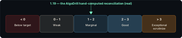
| Annualized Sortino | Verdict | Notes |
|---|---|---|
| < 0 | Below target | Strategy underperforms the target return on a downside-risk-adjusted basis. Stop. |
| 0 – 1 | Weak | Equivalent to Sharpe below ~0.7. Marginal edge; execution costs likely flip it negative. |
| 1 – 2 | Marginal | Covers costs but limited margin. Equivalent to Sharpe ~0.7–1.4 for normal strategies. |
| 2 – 3 | Good | Target range for retail systematic strategies. Comparable to Sharpe 1.4–2.1. |
| > 3 | Exceptional — scrutinize | Often indicates look-ahead bias, near-zero downside observations, or overfitting. |
code-examples.ts.The √2 rule: For normally distributed returns, Sortino ≈ 1.41 × Sharpe. If your Sortino is 3× or 4× your Sharpe, the strategy has significant positive skew (or a methodology error). If your Sortino sits only marginally above your Sharpe (well under the 1.41× a normal distribution implies), the strategy has negative skew — it looks safer on total volatility but carries hidden tail risk. Sortino falling below Sharpe instead signals a negative excess return (a losing strategy), not skew.
Python Implementation
import math

def sortino_ratio(returns: list[float], risk_free_rate: float = 0.0) -> float:
    """
    Compute the period Sortino Ratio (not annualized).

    Args:
        returns:         list of period returns as decimals (e.g., 0.01 for 1%)
        risk_free_rate:  period target / minimum acceptable return (MAR)

    Returns the Sortino Ratio for the period. Multiply by an annualization
    factor to get the annualized Sortino.
    """
    n = len(returns)
    if n < 2:
        raise ValueError("Need at least 2 data points")

    mean_r = sum(returns) / n
    excess  = mean_r - risk_free_rate

    # Downside deviation: only returns below MAR contribute
    downside_sq  = sum(min(r - risk_free_rate, 0) ** 2 for r in returns)
    downside_std = math.sqrt(downside_sq / (n - 1))  # sample denominator

    if downside_std == 0:
        return float("inf") if excess > 0 else 0.0
    return excess / downside_std


ANNUALIZATION = {
    "daily":   math.sqrt(252),
    "weekly":  math.sqrt(52),
    "monthly": math.sqrt(12),
    "annual":  1.0,
}

def annualized_sortino(returns: list[float], periodicity: str = "daily",
                         risk_free_rate: float = 0.0) -> float:
    factor = ANNUALIZATION.get(periodicity, ANNUALIZATION["daily"])
    return sortino_ratio(returns, risk_free_rate) * factor
Example: Comparing Sharpe and Sortino on a Trend-Following Strategy
import numpy as np

# 252 daily returns from a trend-following strategy (positive skew)
daily_returns = np.array([...])  # your actual return array

sharpe = annualized_sharpe(daily_returns.tolist(), periodicity="daily")
sortino = annualized_sortino(daily_returns.tolist(), periodicity="daily")

print(f"Annualized Sharpe:  {sharpe:.3f}")
print(f"Annualized Sortino: {sortino:.3f}")
print(f"Sortino/Sharpe:     {sortino/sharpe:.2f}x  (expect ~1.41 for normal returns)")
# A ratio >> 1.41 confirms positive skew in the return distribution
When Sortino and Sharpe Diverge
The gap between Sortino and Sharpe is a diagnostic tool. For a symmetric (near-normal) return distribution the ratio is ≈ √2. Large deviations signal structural skew:
- Sortino >> √2 × Sharpe (positive skew): The strategy has frequent small losses and occasional large gains — the classic trend-following or long-options profile. Upside runs inflate Sharpe's volatility denominator without representing risk. Sortino correctly ignores them. Use Sortino as the primary metric here.
- Sortino ≈ √2 × Sharpe (near-normal): Consistent with mean-reversion, equity long-only, or diversified multi-strategy. Either metric is reliable; Sharpe is sufficient.
- Sortino < Sharpe (negative excess return): Occurs when the strategy's excess return is negative — the same negative numerator divided by the smaller downside denominator (σD ≤ σ) becomes more negative, so Sortino drops below Sharpe. For a losing strategy this is expected, not an error. For a profitable strategy, Sortino < Sharpe would indeed signal a computation bug — check that you used the same annualization factor and denominator convention (n−1) for both.
Option-selling paradox: Strategies that systematically sell options (e.g., covered calls, cash-secured puts) often have excellent Sharpe and Sortino in calm markets. The premium harvesting produces steady small gains with low observed volatility. Both ratios collapse during volatility events when short gamma positions blow up. Neither Sharpe nor Sortino captures tail risk — use max drawdown and CVaR (Conditional Value at Risk) as complementary metrics.
Sortino vs. Other Risk Metrics
| Metric | What it penalizes | When to prefer it |
|---|---|---|
| Sharpe Ratio | Total volatility (up and down) | Default choice; symmetric payoff strategies; comparing strategies with similar skew |
| Sortino Ratio | Downside volatility only | Trend-following, long volatility; any strategy with known positive skew |
| Calmar Ratio | Max drawdown (not volatility) | CTA-style funds; strategies where drawdown depth matters more than daily vol |
| Information Ratio | Tracking error vs. benchmark | Long-only equity strategies benchmarked against an index |
Best practice is to report Sharpe, Sortino, and max drawdown together. Sharpe captures average vol efficiency; Sortino reveals skew direction; max drawdown anchors the actual pain experienced. A strategy with high Sharpe but Sortino << √2 × Sharpe has negative skew and deserves additional scrutiny. AlgoDrill's calculator computes all three simultaneously from your return series.
Failure Modes: When Sortino Misleads
- Too few downside observations: Downside deviation is estimated from the subset of returns below T. If the strategy rarely loses in the sample (e.g., 10 downside observations out of 252), the downside deviation estimate is highly unstable. A Sortino of 8.0 computed on 10 downside observations is statistically indistinguishable from 2.0 — the confidence interval is enormous. Always report the number of downside observations alongside the ratio.
- Regime-conditional downside: A strategy that avoids drawdowns in a bull market may accumulate massive downside deviation in a bear market. A Sortino computed on a single up-trend will not reflect performance across regimes. Use rolling-window Sortino (e.g., 12-month lookback rolling monthly) to track how the ratio evolves across market conditions.
- Target rate sensitivity: Changing T from 0 to the daily risk-free rate (e.g., 0.02% with T-bills at 5%) can shift Sortino significantly. A strategy with many returns just above 0 but below the risk-free rate will show a much worse Sortino under the second convention. Reports without a stated T are not reproducible.
- Look-ahead bias: Identical to the Sharpe failure mode — any use of future data in signal construction dramatically inflates both Sharpe and Sortino. One tick of look-ahead on a high-frequency strategy can produce a Sortino of 20+ from pure noise.
- Short sample: The same Bailey-López de Prado sampling uncertainty that affects Sharpe applies to Sortino. Treat any Sortino computed on fewer than 60 daily observations (with at least 20 downside observations) as a pilot signal, not a firm conclusion.
Sortino and Position Sizing
Like the Sharpe Ratio, Sortino does not directly determine position size — that is the Kelly Criterion's domain. The two metrics complement each other: evaluate whether the strategy has any edge worth sizing (Sharpe ≥ 1.0 or Sortino ≥ 1.4 as a rough gate), then use Kelly to determine the optimal fraction. A high Sortino with a low Sharpe suggests a positively-skewed strategy where Kelly sizing should account for the asymmetric return distribution rather than assuming normality.
The practical sequence: compute Sharpe and Sortino to evaluate strategy quality; use the Sortino-to-Sharpe ratio to diagnose skew direction; apply Kelly with an appropriate distribution assumption; monitor max drawdown to confirm the Kelly fraction is not exceeding psychological limits.
Frequently Asked Questions
- What is a good Sortino Ratio for algorithmic trading?
- A Sortino Ratio above 2.0 is generally considered good for a live trading strategy; above 3.0 is exceptional and warrants scrutiny for look-ahead bias or overfitting. For symmetric return distributions the Sortino is roughly √2 (≈1.41) times the Sharpe, so a strategy with Sharpe 1.0 should show Sortino near 1.4. Values below 1.0 suggest the strategy earns insufficient return relative to its downside risk.
- How is the Sortino Ratio different from the Sharpe Ratio?
- The Sharpe Ratio divides excess return by total volatility — upside and downside are penalized equally. The Sortino Ratio divides excess return by downside deviation only — returns that fall below the target rate. For strategies with positively-skewed returns (trend-following, long volatility), Sortino is significantly higher than Sharpe because the large upside runs are not counted as risk.
- What target return should I use in the Sortino Ratio?
- Most practitioners use 0 or the annualized risk-free rate converted to the period frequency (T-bill yield ÷ 252 for daily). Using 0 simplifies interpretation and is the industry default for strategy comparison. Using the risk-free rate is theoretically correct for evaluating whether the strategy compensates for its downside risk above cash. Always report which convention you used — the results are not comparable across publications that disagree on T.
- How do I annualize the Sortino Ratio?
- Multiply the period Sortino by the square root of the number of periods per year: ×√252 for daily returns, ×√52 for weekly, ×√12 for monthly. The square-root rule applies identically to Sortino and Sharpe — both assume i.i.d. returns in the annualization step. The only difference between the two is the denominator (downside deviation vs. total standard deviation).
- Why is my Sortino Ratio higher than my Sharpe Ratio?
- This is expected and correct. Downside deviation (the Sortino denominator) is always less than or equal to total standard deviation (the Sharpe denominator) because it counts only returns below the target. For a symmetric normal distribution, downside deviation ≈ σ/√2, so Sortino ≈ Sharpe × √2 ≈ 1.41 × Sharpe. A large Sortino-to-Sharpe gap signals positive return skew — typical of trend-following strategies.
- What does a very high Sortino Ratio mean in backtesting?
- A Sortino above 5.0 in a backtest almost always indicates a methodology artifact. Common causes: look-ahead bias; too few downside observations (near-zero downside deviation inflates the ratio arbitrarily); survivorship bias; or extreme overfitting. Check the number of periods where r < T before trusting any very high Sortino figure — fewer than 20 downside observations makes the estimate statistically meaningless.
Run the Sortino Ratio calculator on your own return series — paste comma-separated returns and get annualized Sharpe, Sortino, and Calmar instantly.
Open Sortino Calculator → Drill Risk Metrics Flashcards →