Statistical Arbitrage: Pairs, Baskets, and Z-Score Entry Rules
Statistical arbitrage (stat arb) trades mean-reverting spreads between cointegrated instruments with a market-neutral objective. The edge is probabilistic: the spread between historically linked instruments tends to revert to its long-run mean after deviations, and that tendency — measured precisely through cointegration, not correlation — is the signal. This page covers the three forms of stat arb, the exact distinction between cointegration and correlation, and a worked z-score entry/exit example.
Strategy archetype cluster:
- Statistical Arbitrage ← you are here
- Pairs Trading — the two-instrument implementation
- Mean Reversion Strategy — single-instrument reversion
- Trend Following — the opposite archetype
What Statistical Arbitrage Is
Stat arb is a relative-value strategy: it does not take a directional bet on whether asset A goes up or down. It bets on the spread — the difference between two or more related prices — reverting to a historical norm. The position is constructed to be approximately market-neutral: a long leg and a short leg offset overall market exposure. If the spread widens beyond its historical mean, stat arb sells the expensive leg and buys the cheap leg; when the spread reverts, both legs move in the strategy's favor regardless of overall market direction.
The word "statistical" is precise: the edge is probabilistic. The spread has a historical tendency to revert, but there is no guarantee it will do so within any given time frame. If the cointegrating relationship between the instruments breaks — because of a structural change, a merger, a policy shift, or sector rotation — the spread can diverge permanently. This distinguishes stat arb from pure (riskless) arbitrage, where the profit is guaranteed by construction.
Three Forms of Stat Arb
| Form | Instruments | Edge source | Key complexity |
|---|---|---|---|
| Pairs arbitrage | Two cointegrated instruments (e.g., two oil majors, two gold ETFs) | Spread mean-reverts to OLS hedge ratio | Finding and testing genuine cointegration (not spurious) |
| Basket arbitrage | A portfolio of N instruments | A stationary linear combination exists across the basket | Portfolio construction, Johansen eigenvector, more legs = more costs |
| Index arbitrage | Index futures vs index components (or index spot vs futures) | Futures basis / mechanical rebalancing flows | Speed (execution window is minutes); capital-intensive |
Cointegration vs Correlation: The Precise Distinction
This is the single most important concept in pairs trading, and it is frequently confused in introductory material.
Correlation measures co-movement of price returns over a window. Two stocks in the same sector may show 0.85 correlation over a year. But correlation tells you nothing about whether the spread between their prices will revert. Both stocks can trend upward together and permanently diverge in price ratio — high correlation the entire time.
Cointegration is the stronger condition. Two price series P_A and P_B are cointegrated if there exists a constant β such that the linear combination P_A − βP_B is stationary — it has no unit root, reverts to a fixed mean, and has bounded variance. This is the mathematical guarantee that the spread will not permanently diverge. Test for it with the Engle-Granger two-step test (statsmodels.tsa.stattools.coint) or the Johansen test for baskets of three or more instruments.
Practical implication: a pairs trader must test for cointegration, not filter by correlation. Finding pairs with high correlation but no cointegration is a common source of spurious stat arb strategies that fail live.
Why Returns Have Been Compressed
Stat arb returns in equities were strongest in the 1990s and compressed significantly through the 2000s as more systematic capital targeted the same signals. The mechanism is straightforward: when more funds apply similar mean-reversion strategies to the same universe, the deviations that generate edge become smaller and shorter-lived. Transaction costs — commissions, bid-ask spread, market impact — then consume a larger fraction of the diminished opportunity. This alpha decay pattern applies to all systematic strategies that become widely known; stat arb is one of the clearest historical examples.
Two responses: (1) move to less-crowded universes (futures cross-hedges, international pairs, alternative data-defined pairs) and (2) improve execution to reduce transaction cost drag. Neither eliminates the compression; they manage it.
Worked Example: Z-Score Entry/Exit on a Pairs Spread
Assume instruments A and B are confirmed cointegrated (Engle-Granger p-value < 0.05). The hedge ratio β is estimated from OLS regression of A prices on B prices over a formation window.
The spread: S(t) = P_A(t) − β × P_B(t)
The z-score over a rolling window of length L (set L to roughly 2× the spread's half-life):
z(t) = (S(t) − mean(S[t-L:t])) / std(S[t-L:t])
| z-score | Signal | Position |
|---|---|---|
| z > +2 | Spread is expensive | Short spread: sell A, buy B (scaled by β) |
| z < −2 | Spread is cheap | Long spread: buy A, sell B (scaled by β) |
| |z| < 0.5 | Spread reverted | Exit position |
| |z| > 3 | Spread widened further — regime risk | Stop-loss or reduce position |
The entry threshold of z = ±2 is a common starting point; the economically optimal threshold depends on transaction costs and the spread's mean-reversion speed (half-life). A spread with a very short half-life tolerates tighter entry thresholds; a slow mean-reverter requires wider entries to make enough profit per trade to cover costs.
Risk not captured by this model: The z-score model assumes stationarity is stable. If the cointegrating relationship breaks, z can diverge without bound — the spread will not revert. Before deploying a pairs strategy, test cointegration on the formation window and monitor it on a rolling basis. A permanent regime change (e.g., one company acquired, sector regulatory change, management change) invalidates the cointegration assumption. Always backtest the strategy through periods where the pair faced structural stress.
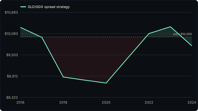
Seeing It in Real Prices: GLD vs GDX
The abstract A/B example above becomes concrete with a real cointegrated pair. Gold bullion (GLD) and gold miners (GDX) are economically linked — but the linkage is not static, which is exactly what this real backtest shows.
Frequently Asked Questions
- What is statistical arbitrage?
- Statistical arbitrage (stat arb) is a market-neutral, mean-reversion strategy that trades the spread between two or more historically linked instruments. The edge is that cointegrated instruments tend to revert to their historical spread relationship after deviations. Stat arb is 'statistical' because the edge is probabilistic, not risk-free: the spread can widen beyond any historical precedent if the cointegrating relationship breaks. It is called arbitrage by analogy with pure arbitrage, not because the profit is guaranteed.
- What is the difference between cointegration and correlation?
- Correlation measures co-movement of price changes over a window — it says nothing about whether the spread between two prices will revert. Two highly correlated instruments can permanently diverge if both are trending. Cointegration is the stronger condition: a stationary linear combination of the two price series exists, meaning the spread itself has no unit root and is pulled back toward a long-run mean by a restoring force. Correlation is necessary but not sufficient for pairs trading; cointegration is the correct statistical test. Use statsmodels.tsa.stattools.coint (Engle-Granger) or the Johansen test to check for cointegration.
- How does z-score entry/exit work in stat arb?
- Form the spread: S = P_A - beta * P_B, where beta is the hedge ratio from OLS regression of P_A on P_B. Compute the rolling z-score: z = (S - mean(S)) / std(S) over a lookback window matched to the spread's half-life. Entry: when z exceeds +2, short the spread (short A, long B); when z falls below -2, long the spread (long A, short B). Exit: when z reverts to 0 (or a tighter threshold such as 0.5). The entry threshold of 2 is a common default; the optimal threshold depends on the half-life and transaction cost structure of the specific pair.
- Why have statistical arbitrage returns compressed?
- More capital targeting the same cointegrated spreads means those spreads are arbitraged away faster. As more systematic funds apply similar mean-reversion signals to the same universe of instruments, the spread deviations that generate the edge become smaller and shorter-lived. Transaction costs then consume a larger fraction of the available profit. This is the general pattern of alpha decay in any systematic strategy that becomes widely known: the edge is real but non-exclusive, and competition for it compresses returns over time.
- What is the difference between pairs, basket, and index arbitrage?
- Pairs arbitrage trades the spread between two cointegrated instruments (e.g., two oil stocks). Basket arbitrage trades the spread between a portfolio of instruments and a benchmark or another basket — the portfolio is constructed to be stationary as a group, even if no individual pair within it is cointegrated. Index arbitrage trades the price discrepancy between an index's spot price and its futures contract (or the aggregate of its components), exploiting mechanical rebalancing flows and futures basis. All three share the core mean-reversion mechanic, but basket and index arb require more sophisticated portfolio construction and hedge ratio calculation.
Drill cointegration tests, z-score mechanics, and strategy archetype trade-offs with AlgoDrill's spaced-repetition flashcards.
Start Strategy Flashcards → Pairs Trading Deep-Dive →