Mean Reversion Strategy: OU Half-Life, Z-Score, and Regime Risk

Mean reversion strategies bet that prices return to equilibrium after deviations. The edge is not discretionary gut feel — it is mathematical: the price series must be stationary (or the spread must be cointegrated), and the half-life must be short enough to generate profit after transaction costs. This page covers the three rule-codifiable entry styles, the Ornstein-Uhlenbeck half-life formula, and the regime conditions under which mean reversion fails.

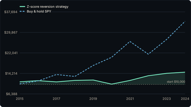
The Mathematical Foundation: Stationarity

A mean-reversion edge requires a stationary price series — one with a finite variance and a pull back toward a stable long-run mean. Most raw price series are not stationary; they are random walks or near-random walks. The first step in any mean-reversion research is testing for stationarity using the Augmented Dickey-Fuller (ADF) test (statsmodels.tsa.stattools.adfuller). An ADF p-value below 0.05 is typically taken as evidence against a unit root (i.e., evidence for stationarity), though the test has low power on short samples.

Single-instrument price series rarely pass the ADF test at the daily or weekly frequency. Mean reversion more commonly appears in: (1) spreads between cointegrated instruments (see Statistical Arbitrage), (2) price ratios or residuals from fundamental models, (3) currency pairs with persistent carry dynamics, and (4) equity/ETF price deviations from a rolling mean when the instrument tracks a mean-reverting factor.

The Ornstein-Uhlenbeck Half-Life

The Ornstein-Uhlenbeck (OU) process is the standard model for mean-reverting price dynamics:

dy(t) = (λ y(t) + μ) dt + dε(t)

The parameter λ (which must be negative for mean reversion) determines the speed of reversion. The half-life — the expected time for a deviation from the mean to shrink by half — is:

half-life = −log(2) / λ

To estimate λ in practice, regress Δy(t) on y(t−1) using OLS; the regression coefficient is an estimate of λ. A positive estimate means the series is not mean-reverting at all. A very small negative λ implies a very long half-life — the strategy will require long holding periods and will struggle to profit after costs. A half-life of 5 days is generally more attractive than one of 50 days at daily frequency.

Three Rule-Codifiable Entry Styles

1. Z-Score Entry

The z-score is the number of rolling standard deviations the current price lies from its rolling mean. Lookback window L should be approximately 2× the half-life.

• Long entry: z < −2 (price statistically cheap)
• Short entry: z > +2 (price statistically expensive)
• Exit: |z| < 0.5 (reversion complete)

Z-score is the most interpretable style because the threshold directly maps to standard deviations from the rolling mean. The +/−2 threshold is a starting point; the optimal entry depends on transaction cost structure and half-life.

2. Bollinger Band Entry

Bollinger bands are a visualization of the same signal: the outer bands sit at ±2 rolling standard deviations from the rolling mean. Entering at the lower band and exiting at the middle band is mechanically equivalent to a z-score strategy with threshold −2 and exit at 0. Chan (Algorithmic Trading, p.71) demonstrates the Bollinger band strategy on the GLD-USO spread pair, noting that the choice of entry z-score directly controls the trade frequency and holding period.

3. RSI-Threshold Entry

The Relative Strength Index (RSI) is a momentum oscillator that measures the ratio of recent up-closes to down-closes over a window. For mean reversion:

• Long entry: RSI < 30 (oversold threshold)
• Short entry: RSI > 70 (overbought threshold)
• Exit: RSI crosses 50 (normalized)

RSI is fully rule-codifiable and automatable. Its weakness as a mean-reversion entry is that RSI can stay below 30 for extended periods during a trend — the same regime-failure problem affects all mean-reversion entries.

Six Points of Nuance

1. Short half-life is necessary but not sufficient

A half-life of 2 days is fast enough to trade profitably after costs at typical commission levels. A half-life of 60 days is borderline; at daily commissions and bid-ask spread, most of the mean-reversion profit is consumed. But a short half-life with no statistical significance (high ADF p-value) is noise, not signal.

2. Lookback window and half-life are coupled

Set the rolling mean lookback window to approximately 2× the half-life. Using a 5-day lookback on a 50-day half-life strategy will produce signals on high-frequency noise, not the true mean-reversion trend. Using a 200-day lookback on a 5-day half-life series creates a non-reactive benchmark that mislabels current fair value.

3. Position scaling improves on binary entry

Scaling position size linearly with the z-score (buy 1 unit per standard deviation of cheapness, up to a cap) produces smoother equity curves than a binary in/out signal at fixed thresholds. The linear scaling approximates the OU strategy's optimal policy under Gaussian assumptions.

4. Mean reversion has negative skew

The return distribution of mean-reversion strategies has a high win rate (most trades close profitably) but negative skew (rare large losses when the spread fails to revert or widens significantly). This is the opposite of trend-following, which has positive skew. The tail risk is a regime change: a trade entered expecting mean reversion into a permanent trend generates an unbounded loss if not capped by a stop.

5. Transaction costs set the floor on half-life

For a strategy to be profitable after costs, the expected profit per trade must exceed the round-trip transaction cost. This sets a minimum on the required half-life and spread of the mean-reversion opportunity. Strategies that look excellent on gross P&L can be unprofitable after realistic cost modeling.

6. In-sample stationarity does not guarantee live stationarity

A series that passed the ADF test in sample may not remain stationary out of sample. Walk-forward validation (see Walk-Forward Analysis) that retests stationarity in each training window is the correct practice.